Uplift Modeling Basics
Uplift modeling is a predictive modeling technique that aims to identify the individuals who are most likely to respond positively to a specific treatment or intervention. This technique is particularly useful in marketing and customer relationship management, where the goal is to target customers who are likely to be influenced by a marketing campaign or offer. By distinguishing between those who are positively influenced by the treatment and those who are not, uplift modeling helps organizations optimize their targeting strategies and maximize the return on investment of their marketing efforts.
Introduction
Uplift Modeling
What is the main issue at hand:
- We cannot do an action & not do an action at the same time to the same person
So what it this modeling approach about:
Uplift modeling is a technique that allows us to identify the subset of objects
- who upon being influenced by an event/action will do some action
- and if not influenced will not do the action
Uplift Modeling Example
Imagine we are selling a product and need to decide to whom we will be advertising, we have some constraints and cannot show it to all target audiences,
- we would like to find clients who will buy the product if they see our advertisement
- and will and not buy it if they don't see it
Uplift Modeling Components
In uplift modeling we need three components:
Have two arrays we will be working with; Treatment Array, Target Array and standard customer related feature matrix
- The Treatment Array is a binary vector, where we have no influence (0) and influenced (1)
- The Target Array is also a binary vector, where we have no action (0) and action is made (1)
- The standard feature matrix (like other machine learning problems) is a matrix that contains features
What to remember
So some important things to note in the context of uplift modeling:
- To model which users will do an action when influenced & users which will not do an action when not influences we need to have aside from a standard feature matrix two additional vectors; Treatment Array (users were identified and interacted with) & the result of our interaction with them, stored in the Target Array
- Having a trained model will enable us to identify on unseen data (without a treatment or target vector) the uplift value for a group for which we have a set of features used in training
- Our aim is to target influencible clients (those who upon being interacted with will commit a target action) and those who can be positively influenced (when not interacted with will not conduct a target action).
Loading Data
Kevin Hillstrom Dataset
Our dataset is available in the sklift library, called Kevin Hillstrom Dataset. You can also try other sample problems shown below:
# Kevin Hillstrom Dataset
from sklift.datasets import fetch_x5, fetch_lenta, clear_data_dir, fetch_megafon, fetch_hillstrom

data = fetch_hillstrom()
Lets introduce ourselves to the dataset we will be using in our notebook, by looking at the description provided with the dataset
This dataset contains 64,000 customers who last purchased within twelve months. The customers were involved in an e-mail test.
- 1/3 were randomly chosen to receive an e-mail campaign featuring Mens merchandise.
- 1/3 were randomly chosen to receive an e-mail campaign featuring Womens merchandise.
- 1/3 were randomly chosen to not receive an e-mail campaign.
During a period of two weeks following the e-mail campaign, results were tracked. Your job is to tell the world if the Mens or Womens e-mail campaign was successful.
Having read the above, lets summarise the important bits:
- We have 64000 customers who recently made a purchase, for these customers we have a matrix of features relevant to each of these customers
- We randomly send emails to these customers (treatment array); we have an array containing a marketing campaign defined subset groupings
- Finally we have a target containing post marketing campaign monitored results (confirmations of whether the email campaign worked or not)
Data Insight
Feature Matrix
Let's also look at the feature matrix available to us:
+-------+---------------+-------+----+------+---------+------+-------+
|recency|history_segment|history|mens|womens| zip_code|newbie|channel|
+-------+---------------+-------+----+------+---------+------+-------+
|     10| 2) $100 - $200| 142.44|   1|     0|Surburban|     0|  Phone|
|      6| 3) $200 - $350| 329.08|   1|     1|    Rural|     1|    Web|
|      7| 2) $100 - $200| 180.65|   0|     1|Surburban|     1|    Web|
|      9| 5) $500 - $750| 675.83|   1|     0|    Rural|     1|    Web|
|      2|   1) $0 - $100|  45.34|   1|     0|    Urban|     0|    Web|
+-------+---------------+-------+----+------+---------+------+-------+
Treatment Array
The treatment array contains text data which we will need to convert into numerical data, we have information about the marketing campaign, in which we roughtly speaking to do one of two things; send an email about the marketing campaign or don't send anything
t.sample(5)

3947       Mens E-Mail
48105      Mens E-Mail
15614      Mens E-Mail
58595        No E-Mail
21571    Womens E-Mail
Target Array
The target contains the result of the email marketing campaign influence and is already in numerical format, it reflects whether the campaign was successful or not
Preprocessing
Problem Simplification
Lets do a little bit of preprocessing and problem simplification. As we saw in the above data, we have three categories in our treatment vector. Lets simplify it to just a binary case and not differentiate the male and female target cases, ie. marketing email has been sent or not sent.
Train Test Splitting
Lets also split the data into training & test subsets, we will need some unseen data to validate our models.
X_train, X_test, y_train, y_test, t_train, t_test = train_test_split(X, y, t, test_size=0.3, random_state=42)
Categorical Feature Treatment
We have to also pay attention to categorical features which are present in our feature matrix, a common and most straightforward approach is to use One Hot Encoding, which will be applied to three columns.
We will fit the one hot encoder on our training dataset, and only apply it to the test dataset
cat_columns = ['history_segment', 'zip_code', 'channel']
enc = OneHotEncoder(sparse=False)

X_train_cat = enc.fit_transform(X_train[cat_columns])
X_train_cat = pd.DataFrame(X_train_cat,
                           index=X_train.index,
                           columns=enc.get_feature_names_out(cat_columns))

X_test_cat = enc.transform(X_test[cat_columns])
X_test_cat = pd.DataFrame(X_test_cat,
                          index=X_test.index,
                          columns=enc.get_feature_names_out(cat_columns))

X_train = pd.concat([X_train_cat, X_train.drop(cat_columns, axis=1)], axis=1)
X_test = pd.concat([X_test_cat, X_test.drop(cat_columns, axis=1)], axis=1)
Modeling Approaches
Now that we have our data ready, lets talk libraries and approaches. There is a commonly used uplift modeling library called scikit-uplift, its based on scikit-learn machine learning models, but modified for uplift modeling. Lets remind ourselves of what the modeling actually wants to achieve:
Abstract
Uplift modeling focuses on predicting the impact of a treatment or intervention on an individual's behavior
scikit-uplift has a number of different approaches for uplift modeling, you can find the models in the following link, we'll look at two of the three approaches used in the library
One Model Approach
Starting with s-learner approach, we train two separate models
- We train a base model with all base features and the treatment vector (w), taking the target vector (y) as our independent variable
- Apply the model (predict) assuming we have interacted with all customers, ie. (t=1 for all customers), and ask to return the probability of a successful outcome (y=1) for this group
- Apply the model (predict) again but assuming that these has been no interaction with any customer (t=0 for all customers)
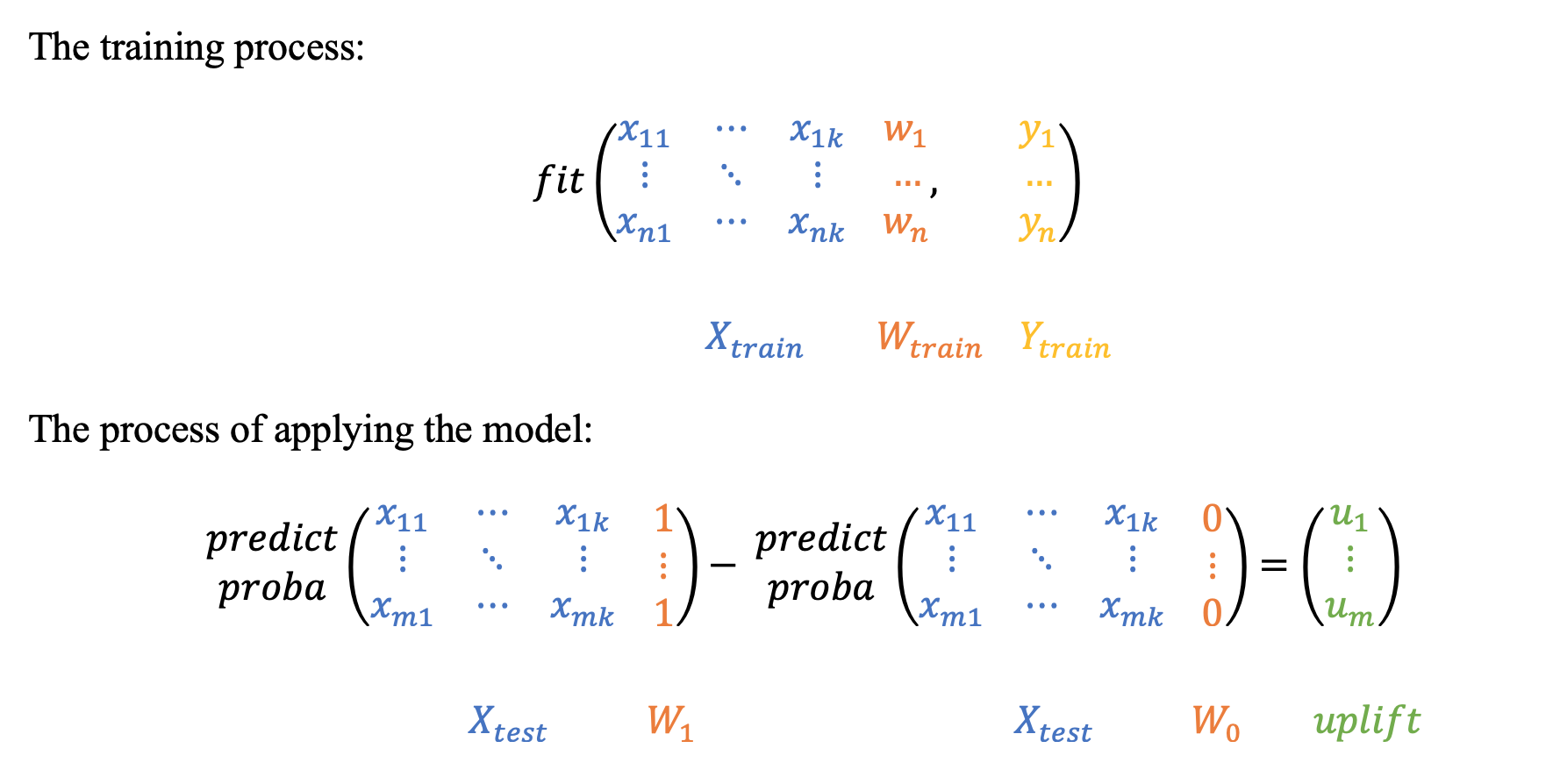
The difference between these two vectors will be taken as our uplift, to be more specific:
model generates uplift scores that represent the estimated impact of a treatment on each individual's behavior
The s-learner model can be used by importing SoloModel from from sklift.models import SoloModel, we just need to specify the base model we will be using in the two models and wrap it with SoloModel. Like other sklearn models, we use fit,predict methods, but with an additional input t_train
name = 'slearner'

base_model = RandomForestClassifier(random_state=42)
uplift_model = SoloModel(base_model)
uplift_model = uplift_model.fit(X_train, y_train, t_train)

# store the uplift values
model_predictions[name] = uplift_model.predict(X_test)
We obtain our uplift values:
Interpretation of Results
- If the results are positive for a particular entry, it indicates that the treatment (email marketing campaign) has a positive effect on this individual and visa versa.
- In terms of magnitude, a larger positive (or negative) uplift score implies a more significant impact of the treatment on the individual's likelihood of a positive outcome.
Two Independent Model Approach
The two model approach, t-learner is similar to a one model approach, however instead of training a single model on all the data, we train two models, on two different subsets of data:
- One for the control group (no interaction, t=0)
- Another for the test group (there was interaction, t=1)
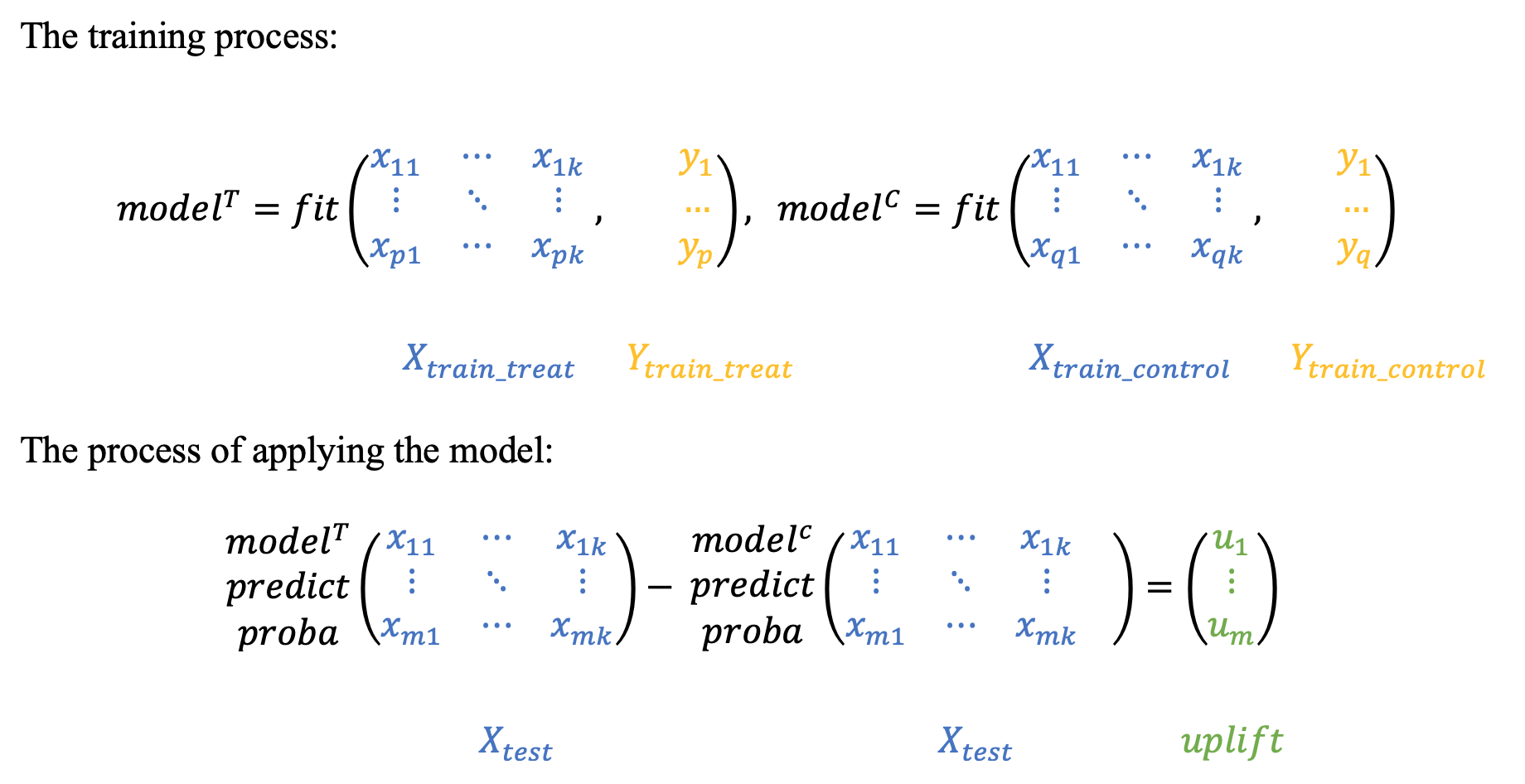
In order to obtain the uplift, we apply the model on the test set like in the s-learner, with the exception that we dont add the additional treatment feature, instead we are using two independent models. The difference in predict_proba between these two models will be our uplift value.
from sklift.models import TwoModels

name = 'tlearner'

# control group
basic_model_control = RandomForestClassifier(random_state=42)

# test group
basic_model_test = RandomForestClassifier(random_state=42)

uplift_model = TwoModels(basic_model_test, basic_model_control, method='vanilla')
uplift_model = uplift_model.fit(X_train, y_train, t_train)

# store the uplift values
model_predictions[name] = uplift_model.predict(X_test)
We obtain our uplift values:
We can also plot the uplift values predicted by both modeling approaches:
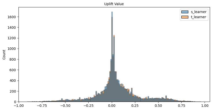
We can notice a very minor binomial tendency in the figure, a large portion of users having a low uplift values around 0-0.25 & a secondary group around 0.3-0.75, in terms of model variation, we can clearly note that t-learner is less concentrated with values at 0 and instead has more values in the region 0-0.25, which would indicate that the model predicts on average that the user is more confident that the user is positively influenced than the s-model
Conclusion
Metric Evaluation
So now that we have obtained our uplift values, we ought to evaluate how well our modeling is. When it comes to uplift modeling problems, we can turn to a metric called uplift@k.
The metric ranges from -1 to 1, where 1 is the best and -1 represents a model that doesnt work. A value of 0 is equivalent to a random model. Values in the range 0.05 to 1 can be considered as working models.
The evaluation methodology is as follows:
- We take k objects with the highest uplift values
- Divide the subset into a contol (t=0) and test (t=1) group
- Evaluate the average target y for each individually
-
Find the difference:
\[ uplift@k = \bar{y}_{k \space test} - \bar{y}_{k \space control} \]\[ \bar{y}_k = \frac{1}{n} \sum_{i=1}^{k}{uplift_i,} \]
There are some other metrics you can look into as well:
- Area Under Uplift Curve
- Area Under Qini Curve
- Weighted average uplift
results = dict()
for model_name, preds in model_predictions.items():

    up_k_best = uplift_at_k(y_true=y_test,
                            uplift=preds,
                            treatment=t_test,
                            strategy='overall',
                            k=0.2)

    results[model_name] = round(up_k_best,4)
What we can conclude is that the t-learner method has a slightly higher metric values compared to s-learer, which indicates that it is a slightly better modeling approach.
Remarks
In this post we looked into a brief introduction into uplift modeling, which is a practical business task for which we can utilise machine learning & use modeling for the prediction/identification of the subset of objects/dataset who upon being influenced by an event/action will do some action and if not influenced will not do the action
We looked at two approaches s-learner & t-learner modeling approaches and tried a sample problem Kevin Hillstrom Dataset
The modeling approaches allow us to predict the lift value, and gives us to understanding how well the particular client is influenced based on historical data, the models can then be used on new unseen data.
We can repeat the process similar to above using some other datasets such as: fetch_x5, fetch_lenta, fetch_megafon.
Thank you for reading!
Any questions or comments about the above post can be addressed on the mldsai-info channel or to me directly shtrauss2, on shtrausslearning or shtrausslearning or simply below!